Institute of Mathematical Geography

Sandra L. Arlinghaus

Introduction

Steiner's problem is that of finding a shortest path joining an arbitrary number of points. The solution is a graph-theoretic tree of minimum length, a 'Steiner tree', and it may include points not given in the original set. It is precisely this latter possibility that distinguishes Steiner's problem from others, such as the travelling salesman problem, although both of these, and other network optimization problems, are NP-complete. Any new point, chosen to reduce total network length joining the original set of points (a 'Steiner point'), may be chosen from an an infinite set of positions. The challenge is to determine how to find these intervening positions.

Here, the power of animation is employed to advantage to offer the reader visual guidance in the spatial process of finding Steiner trees. Example is chosen from previous work done by the author (Arlinghaus, 1977; Arlinghaus, 1989). In these earlier documents, images are only static and they quickly become visually complex; so too, associated proofs of theorems become notationally complex. Animation unravels that complexity.

The Case of Three Given Points

In the case of three given points, V1, V2, and V3, form a triangle from the points (Figure 1). The Steiner Tree will either follow along two sides of the triangle itself, as a 'degenerate' tree, or an extra point will produce a new network shorter than following the two shortest sides. There is no unique construction for finding the extra Steiner point; a number of them exist. The one presented here is due to Hoffman (Figure 1) and is chosen because it is the one that appeared to generalized geometrically in a somewhat straightforward manner (Coxeter, p. 21).

The animation in Figure 1 opens with the set of three points displayed. The next frame forms a triangle on these three points. The third frame identifies side V1V2 of the triangle by coloring it magenta. A subsequent sequence of faster moving frames rotates the magenta side, through 10 degree increments, to a final position rotated through V1 60 degrees from V1V2 to V1V2'. The next frame inserts the circle that circumscribes the triangle V1V2V2'; that circle is presented in cyan at 25% opacity. Following that, the line V2'V3 is drawn, in cyan. The point S, the Steiner point, is introduced in the next frame as the intersection of the circumcircle and the line V2'V3. From there, S is joined, using lighter weight red lines, to each of V1, V2, V3 to produce the Steiner tree within the triangle. The central angles at S are all 120 degrees. Finally, the triangle is removed to reveal only the Steiner tree on these three points. Then, the scene dissolves back to the starting arrangement. The proofs, explaining why this construction works, and when it is necessary, are available in a variety of references (Coxeter, 1961; Cockayne, 1967; Melzak, 1961; Gilbert and Pollak, 1968; Werner, 1968 and 1969). The ones that most closely match the visual display in this section and subsequent sections are in works by the author (Arlinghaus, 1977 and 1989).

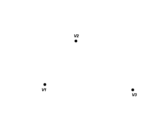Figure 1 .

Two Higher Order Steiner Trees

In this section, the general labeling and coloring scheme in the figures is that suggested by the case of three given points: magenta lines are derived by rotation through 60 degrees and cyan circles are circumcircles associated with that rotation. Lines are used to intersect cyan circles to determine Steiner point positions. Finally, Steiner points are joined to each other and to given points at angles of 120 degrees, using lighter weight red lines, to produce a Steiner tree. Subtle variations, in label position, density of opacity, and so forth are used as emphasis without clutter.

The Case of Four Given Points

A non-degenerate Steiner tree on four given points has two new Steiner points, S1 and S2, introduced. Figure 2 illustrates the manner of construction for this sort of tree.

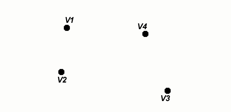
Figure 2.

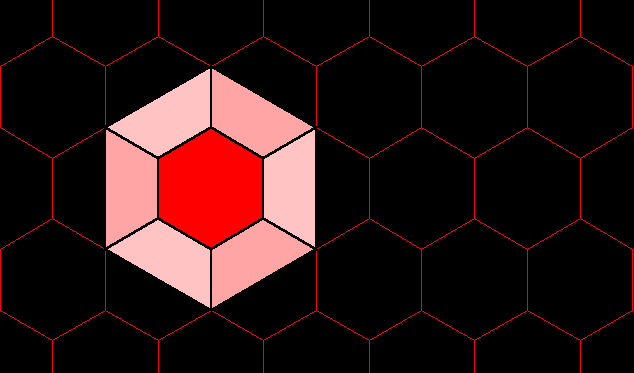
The Case of Six Given Points

A non-degenerate Steiner tree on six points has four new points introduced. In Figure 3, the construction involves reduction to a previous case: reduction of the hexagon to the triangle. The circumcircle with 10% fill, rather than 25% fill, aids in this reduction.

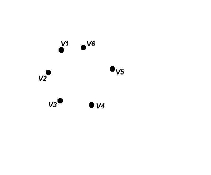
Figure 3.

A Closer Look at the Six Point Case

The construction show in Figure 3 is for a hypothetical distribution of six points, designed to illustrate process. In the real world, the spacing among six points, chosen for geographical or other reasons, might not produce such a display. Now, consider a set of six locations at the edge of Lake Michigan and reflect on various ways that they might be joined--shipping route constraints, weather-related issues, or supply and demand needs at various ports. Figure 4 illustrates the patterns of linkage, each a Steiner tree of prescribed connection pattern, that might emerge (Arlinghaus, 1977).

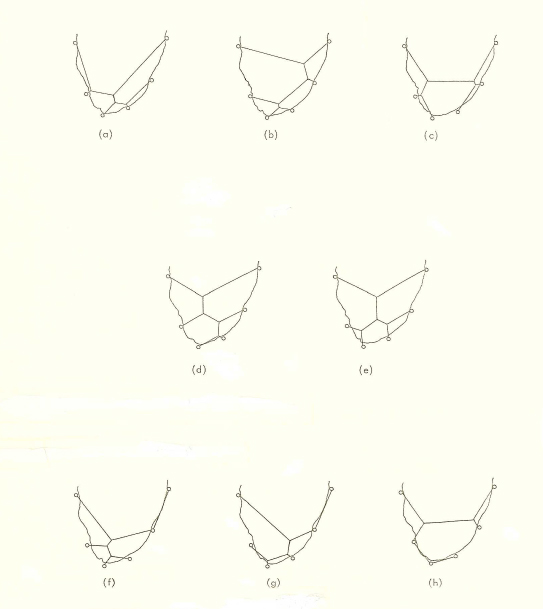
Figure 4. Arlinghaus, 1977.

The sequence of figures below shows an animation for each of these eight figures, with figure number to correspond to the labeling in Figure 4. In these, vertex labels are by now assumed to be familiar and are left off to expose the construction more clearly. Some networks are full, requiring the full complement of new points, while others are partially degenerate. Variation in the animation is designed to focus emphasis.

Figure 4a.

Figure 4b.

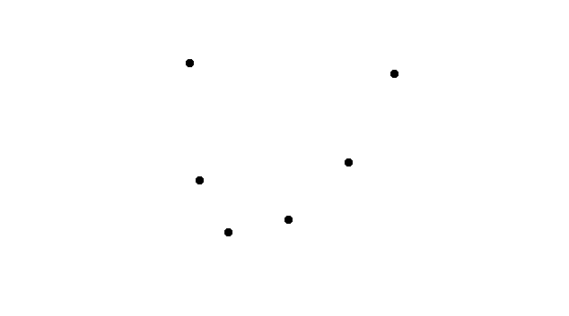
Figure 4c.

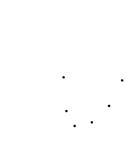
Figure 4d.

Figure 4e.

Figure 4f.

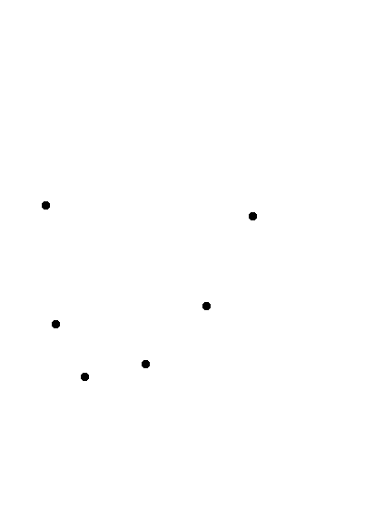
Figure 4g.

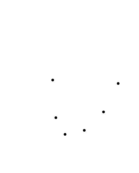
Figure 4h.

Geometric views that become complex can be improved, in terms of comprehension, with animation. Older texts can be made to come alive; more recent ones can be brightened (eBook materials associated with Arlinghaus and Kerski, 2013); most important, animation can do more than enhance existing research--as it opens better or new vistas, it can guide it!

References

Arlinghaus, Sandra L. 1977. On Geographical Network Location Theory. Ph.D. Dissertation, Department of Geography, The University of Michigan.

Arlinghaus, Sandra L. 1989. An Atlas of Steiner Networks. Monograph 9. Ann Arbor: Institute of Mathematical Geography.

Arlinghaus, Sandra L. and Kerski, Joseph. 2013. Spatial Mathematics: Theory and Practice through Mapping. Boca Raton: CRC Press.

Coxeter, H. S. M. 1961. Introduction to Geometry. New York: John Wiley & Sons.

Cockayne, 1967. On the Steiner problem, Canadian Mathematical Bulletin, 10, 431-450.

Melzak, Z. A. 1961. On the problem of Steiner, Canadian Mathematical Bulletin, 4, 143-148.

Gilbert, E. N. and Pollak, H. O. 1968. Steiner minimal trees, SIAM Journal of Applied Mathematics, 16, 1-29.

Werner, C. 1968. The role of topology and geometry in optimal network design, Papers of the Regional Science Association.

Werner, C. 1969. Networks of minimum length, The Canadian Geographer, XIII, 1, 47-69.