To see how self-similarity might generate street pattern, consider the application of a V-shaped generator, applied to a square initiator, to generate successive stages of finer and finer grid pattern (Figure 1, Arlinghaus 1985, 1990).    The animations of Figure 1 illustrates the process through successive stages of generator application and scaling.  Figure 1a illustrates the general process while Figure 1b suggests how to visualize the detail of application of the fractal generator. The limiting position of such space-filling occurs when this iteration of transformation is carried out infinitely.  Using Mandelbrot’s characterization of fractional dimension, the space-filling is captured as D = log(n)/log(), where n is the number of generator sides and K is the number of self-similar regions. Thus, in the case of Figure 1, D = log(2)/log() = 2. When the process is carried out infinitely, the entire area over which it is carried out becomes filled with network edges.  In order to suggest network scaling and pattern, one would wish to truncate the iterative process and stop it after a finite number of steps, perhaps determined by smallest parcel size according to zoning category.

Figure 1a.  A style of hierarchy generated through self-similarity applied to a square initiator. D = 2.  General iteration sequence.

Figure 1b.  Visualization of detail of generator application in Figure 1a.

Changing the generator, but keeping the same initiator (a square) produces a different pattern (Figure 2).  The animations of Figure 2 illustrates the process through successive stages of generator application and scaling.  Figure 2a illustrates the general process while Figure 2b suggests how to visualize the detail of application of the fractal generator.  Here, in the infinite process, the fractional dimension is D = log(3)/log() = (2/3)*log(3)/log(2) = 1.0619248.  The choice of the three-sided generator produced a pattern shaped similarly to the choice of the two-sided generator but did so in a much less compact manner.  Hence, the space-filling of the lines and associated fractional dimension are less than in the previous case, suggesting orientation of street pattern to parcel in yet another manner.  Again, though, to realize the model in relation to street networks and parcels, the iteration would need to be truncated, presumably in relation to the urban character of the space under consideration.

Figure 2a.  A style of hierarchy generated through self-similarity applied to a square initiator. The dotted lines show the polygon generated (or given in the previous state).  The solid lines show the generated edges.  The dashed lines are inferred (but not generated) pattern.  Thus, the value of D = 1.0619248 applies only to the generated (solid) pattern.  General iteration sequence.

Figure 2b.  Visualization of detail of generator application in Figure 2a.

Alternative Geometric Generation of Fractals:  Eigenvalue Geometry

One method of making direct calculations of fractional dimension relies on using a generator applied at successive scales to an initial shape. Successive generator application to new self-similar shapes creates an infinite process that converges to some finite value as a fractional dimension.  The previous section showed two examples.  Generator selection, to produce a desired outcome (pattern or number) is an art.

In this section, we reconsider the example of Figure 2 generated above with respect to different underlying geometric processes.  With generator scaling and creative generator shape selection, as above, only an envelope of the associated pattern is generated.  Advantages of the strategy suggested below are:

·         The full pattern, and not merely its envelope, is generated.

·         A systematic geometric process with roots in linear algebra may offer interesting related connections.

A scaling effect is evident in the process above as the generator is successively scaled to fit polygon sides.  An alternative procedure for generating the fractal sequence of Figure 2 employs a single shape, a “4-star graph,” that when translated across the plane creates the same pattern as in Figure 2. The sequence of images in Figure 3 illustrates the process: begin with a 4-star graph (Figure 3a), apply a shift it to the right (Figure 3b), continue stretching to shift the image in the same direction as the original transformation (Figure 3c). Then, using a shift orthogonal to the first one, apply it to a 4-star graph to shift it (Figure 3d), continue stretching to shift the image in the same direction as the original transformation (Figure 3e). Finally, use the two shift directions  to fill in the rest of the space (Figure 3f).

In a geometric interpretation of a linear algebra context, the shift directions function as  eigenvectors of a transformation to create the pattern when they are applied to a 4-star graph. The eigenvalues of the transformation are the amounts the eigenvectors are stretched or shrunk. In this example, one might consider each basic eigenvector to have length 1, in which case other eigenvalues would be the set of positive and negative integers. If, however, this synthetic geometric form is superimposed on some underlying coordinate system, then the eigenvalues might be different, although still integral, multiples of the basic one. Notice that the visualization of Figure 3 shows where these vectors are “lurking” in Figure 2—they are the edges of the polygon to which the generator is applied!

Figure 3. a.  Initial 4-star. b.  Vector to shift pattern. c.  Successive application of vector d.  Vertical shift. e.  Successive application of vertical vector. f.  Use of the pair of vectors to fill in pattern.

The sequence in Figure 3 generates the first layer of pattern. To illustrate how to create a subsequent layer, and all others, focus on a single generated polygon (teragon) from Figure 3f (shown in Figure 4a). Begin, again, by introducing a single small 4-star graph (Figure 4b). Apply a vector to transform it (Figure 4c). Continue the application in the same direction, positive or negative (Figure 4d). Apply an orthogonal vector to move the 4-star graph (Figure 4e). Continue the application of that vector in positive and negative directions (Figure 4f).  What causes the shifts here are the orthogonal vectors; in this case, the art comes in selecting the initial pattern, the 4-star, rather than in selecting the generator.  Here, generators are directed straight line segments.

Figure 4. a.  Focus. b.  Initial 4-star. c.  Vector to shift pattern. d.  Successive application of vector. e.  Orthogonal shift. f.  Successive application of orthogonal vector.

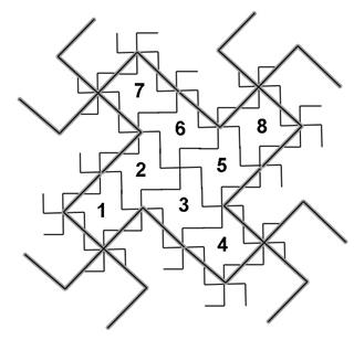
Combinations of the vectors in Figure 4 expand pattern to fill space. Figure 5a shows this space filling together with the pattern of basic vectors in relation to each other: both orientation and length. Figure 5b shows that the process creates 8 scaled-down teragons self-similar to the first teragon.  Notice that the full pattern, and not merely its envelope, is generated by this process.  This alternative strategy is faithful to the initial ideas involving self-similarity.

Figure 6 shows that the classical method for fractal generation using a generator on an initiator yields the same result as using shifts induced by vectors.

Figure 6.  Figure 5b, from the vector approach, is overlain on Figure 2c from the classical approach.

The ideas suggested in the iteration sequences in Figures 4 and 5 might be viewed as broadly  similar to downtown planning:  fill an area with buildings as allowed by zoning, and put in as many roads as possible to facilitate movement; superimpose a park if desired, but as an overlay on fundamental strategy; and, use the value of D = 2 as the upper bound beyond which space-filling by roads is not permitted, except in situations where there are multiple vertical layers of street network (beyond the scope of this broad suggestion).

One might determine, in advance, the extent of permitted space-filling by a road network as, perhaps, a new class of zoning. Traditional zoning basically mandates such filling by buildings and land use types. Then, one might use the appropriate fractal dimensions, generated as absolute (rather than as relative) values based on the iteration of self-similar generators applied to an initiator. Figure 7 illustrates how one might interpret these ideas in a simple landscape, much as Burgess offered a simple example, based on the mathematics readily available to him.

In the central ring of Figure 7, the street pattern envelope is generated by the iteration sequence of Figure 1; the initiator is shaded a solid yellow color and is identical to the initiator in Figure 1. The second frame in the animation sequence in Figure 1 is displayed in Figure 7 as a blue shape.  Grid pattern is filled in with fractal iteration, as suggested in the animation of Figure 1.  Here, the sequence employed leads to D = 2 when carried out infinitely (lines would fill everything).  It is truncated here after two steps and its edges form the suggested road network with streets becoming successively narrower as the pattern iterates.

In the outer ring of Figure 7, the street pattern envelope is generated by the iteration sequence of Figure 2; The initiator is shaded solid orange.  The second from of the animation yields the brown shape--follow the generator edges with your eye.  Again, narrower streets come from the edges of smaller (later) iterates.   Grid pattern is filled in through successive generator application.  Here the sequence employed leads to D = 1.0619248 when carried out infinitely (there would be gaps between lines—some space would not be filled).

The two iteration sequences displayed in Figure 7 mesh quite well at the boundary separating one region from the other. Larger roads from the core region flow naturally into roads in the rim. Some of the more local angled roads in the core region flow into the intersections of larger roads along the ring perimeter. These locales might be natural places to install traffic circles (avoiding costly traffic lights). In Figure 7, stars suggest locations for traffic rotaries, with the largest ones marking locations where the largest roads come together, and so forth, creating a hierarchy of rotaries marked by stars of various sizes.  Others of the more local angled roads do not continue into the outer ring. These roads become natural cul-de-sacs, and offer privacy or low-profile needs to specific land use types in the core.  In Figure 7, circles mark the locations of cul-de-sacs arising naturally in the shift of the underlying grid dimension. Zoning might follow the form created by the meshing or failure to mesh of the underlying geometry, giving parcels on cul-de-sacs special zoning that reflects privacy or security concerns.

Figure 7. Fractally-bounded parcel and road pattern development.  The iteration sequence of Figure 1 generates the road network in the central circle.  The iteration sequence of Figure 2 generates the road network in the outer ring.

The two-ring pattern displayed in Figure 7 might of course be extended to include more rings, reflecting variety in zoning types. In such extension, traffic circles/rotaries would emerge at boundaries.  Cul-de-sacs would emerge in moving from one ring to another, and, again, zoning patterns might follow their appearance.

REFERENCES CITED AND RELATED READING

Arlinghaus S., 1985, Fractals take a central place, Geografiska Annaler, Journal of the Stockholm School of Economics, 67B, pp. 83-88.

Arlinghaus, S., 1990, Fractal geometry of infinite pixel sequences: “Super-definition” resolution? Solstice: An Electronic Journal of Geography and Mathematics, Volume I, Number 2. Ann Arbor: Institute of Mathematical Geography. http://www.imagenet.org. Persistent URL: http://deepblue.lib.umich.edu/handle/2027.42/58219

Arlinghaus S., Griffith D. 2010. Mapping it out! A contemporary view of Burgess’s concentric ring model of urban growth, Solstice, XXI (2), www.mylovedone.com/image/solstice/win10/ArlinghausandGriffith.html

Arlinghaus S., Nystuen J., 1990, Geometry of boundary exchanges: Compression patterns for boundary dwellers, The Geographical Review, 80, 1, pp. 21-31.

Arlinghaus S., Nystuen J., 1991, Street geometry and flows, The Geographical Review, 81, 2, pp. 206-214.

Arlinghaus S., Arlinghaus W., 1989, The fractal theory of central place hierarchies: a Diophantine analysis of fractal generators for arbitrary Löschian numbers, Geographical Analysis: an International Journal of Theoretical Geography, 21, 2, pp. 103-121.

Batty M., Longley P., references listing: http://www.casa.ucl.ac.uk/people/MikesPage.htm

Benguigui L., Daoud M., 1991, Is the suburban railway system a fractal? Geographical Analysis, 23, pp. 362-368.

Boots, B.N. and G.F. Rayle, “A conjecture on the maximum value of the principal eigenvalue of a planar graph”, Geographical Analysis, 23(3), 1991, 276-282.

Cardillo, A., S. Scellato, V. Latora, and S. Porta. 2006. Structural properties of planar graphs of urban street patterns, Physical Review E, 73: 066107-1 - 066107-8.

Coxeter H., 1965, Non-Euclidean Geometry, University of Toronto Press, Toronto.

Elert G., 1995-2007, About Dimension, The Chaos Hypertextbook, http://hypertextbook.com/chaos/33.shtml

Griffith, D. 2004. Extreme eigenfunctions of adjacency matrices for planar graphs employed in spatial analyses, Linear Algebra & Its Applications, 388: 201-219.

Griffith, D. 2000. Eigenfunction properties and approximations of selected incidence matrices employed in spatial analyses, Linear Algebra & Its Applications, 321: 95-112.

Griffith, D., and S. Arlinghaus. 2011. Urban compression patterns: fractals and non-Euclidean geometries inventory and prospect, Quaestiones Geographicae.

Griffith D., Vojnovic I., Messina J. 2010. Distances in residential space: implications from estimated metric functions for minimum path distances, unpublished paper, School of Economic, Political and Policy Sciences, University of Texas at Dallas.

Grünbaum B., Shephard G., 1987, Tilings and Patterns, W. H. Freeman, New York.

Hausdorff and Besicovitch, historical reference: http://en.wikipedia.org/wiki/Hausdorff_dimension

Kansky, K. 1963. Structure of Transportation Networks. University of Chicago, Department of Geography.

Kim, K., L. Benguigui, and M. Marinov. 2003. The fractal structure of Seoul’s public transportation system, Cities, 20: 31-39.

Krause E., 1975, Taxicab Geometry, Addison-Wesley, Menlo Park, CA.

Li, J., X. Wang, and Q-S Guo. 2002. Research on fractal characteristics of urban traffic network structure based on GIS, Chinese Geographical Science, 12: 346-349.

Lu, Y., and J. Tang. 2004. Fractal dimension of a transportation network and its relationship with urban growth: a study of the Dallas-Fort Worth area, Environment and Planning B, 31: 895-911.

Mandelbrot B., 1983, The Fractal Geometry of Nature, W. H. Freeman, New York.

Ord J., 1975, Estimation methods for models of spatial interaction, Journal of the American Statistical Association, 70, pp. 120-126

Park, Robert I. And Burgess, Ernest W. 1925. The City. Chicago: The University of Chicago Press.

Rodin V., Rodina E., 2000, The fractal dimension of Tokyo's streets, Fractals, 8, pp. 413-418

Shen G., 1997, A fractal dimension analysis of urban transportation networks, Geographical & Environmental Modelling, 1, pp. 221-236.

Telecs, A. 1990. Spectra of graphs and fractal dimensions I, J. of Theoretical Probability, 8: 77-96.

Telecs, A. 1995. Spectra of graphs and fractal dimensions II, Probability Theory and Related Fields, 85: 489-497.

Thrasher, F. M. 1923-1926. Chicago’s Gangland Map. http://www.lib.uchicago.edu/lib/public/full_screen.html?http://www.lib.uchicago.edu/e/su/maps/chisoc/G4104-C6E625-1926-T5

Wikipedia, Fibonacci Coding: http://en.wikipedia.org/wiki/Fibonacci_coding.