| SOLSTICE: An Electronic Journal of Geography and Mathematics. (Major articles are refereed; full electronic archives available). Persistent URL: http://deepblue.lib.umich.edu/handle/2027.42/58219 |
 |
| SOLSTICE: An Electronic Journal of Geography and Mathematics. (Major articles are refereed; full electronic archives available). Persistent URL: http://deepblue.lib.umich.edu/handle/2027.42/58219 |
|
 Educational Research Collaboration Part 2 Sandra L. Arlinghaus, Ph.D. and Joseph J. Kerski, Ph.D. "I
believe that man will not
merely endure, he will prevail."
IntroductionWilliam Faulker, Nobel Prize Acceptance Speech, December 10, 1950. As exciting new vistas open doors in both geographical and mathematical visualization, it may be easy to get caught up in the focus within one discipline or the other. The richness that comes from interplay between disciplines can get cast aside, only to be rediscovered much later when single disciplines have matured and are looking for the fresh and new, beyond original disciplinary boundaries. When such loss occurs at the research level, it is disappointing because much creative activity can slow down while more conventional activity plays out its course within established, comfortable, and conventional limits. When such loss occurs in the education of children it can be far more dramatic, indeed tragic, as generations of future citizens, voters, municpal authorities, students, researchers, and teachers may become trapped in curricular conventions of a particular decade. A number of scholars, in wide-ranging fields, have long seen this difficulty. It becomes perhaps more pronounced now with the technological revolution within which so many projects, scholarly and educational alike, are set. One form such entrapment may take is in the confusion of toolkits with concepts. Duane Marble recently characterized this difficulty quite clearly: "Confusing science with the tools of
science is an increasing problem in our
discipline. Geographic science
forms the basis for spatial and spatiotemporal
analysis. Over the past
few decades we have developed a complex tool kit
that we refer to as
GIS. The tool kit exists for two reasons: the
advancement of geographic
science and to effectively apply many of the
concepts of geographic
science to the solution of a large number of the
problems of our
society. You cannot make effective use of GIS
tools unless you
understand geography.
There is also some confusion in the words that we use to talk about GIS. "Geospatial" is a term that was created by people outside of Geography who were uncomfortable with the "Geographic" part of Geographic Information Systems. "Geomatic" is a Canadian term that was set forth as a compromise term between the geography/cartography and surveying communities of that nation. It also fits well into their English/French language situation. GIS tools have been highly successful and have opened spatial and spatiotemporal doors in many areas, both scientific and practical, that had been ignoring spatial and spatiotemporal factors since they were too difficult to deal with using the traditional, analog tool kit that we lived with for so long." We have both been interested, for at least a part of our careers, in helping to bridge the interdisciplinary gap between geography and mathematics (particularly geometry). One reflection of our interest appears in a previous article (the first in the MatheMaPics set) while another appears in a forthcoming book (Spatial Mathematics: Theory and Practice through Mapping). |
|||||||||||||||||||||||||||||||||||||||||||||||||||||||||||||||||||||||||||||||||||||||||||||||||||||||||||||||||||||||||||||||||||||||||||||||||||||||||||||||||||||||||||||||||||||||||||||||||||||||||||||||||||||||||||||||||||||||||||||||||||||||||||||||||||||||||||||||||||||||||||||||||||||||||||||||||||||||||||||||||||||||||||||||||||||||||||||||||||||||||||||||||||||||||||||||||||||||||||||||||||||||||||||||||||||||||||||||||||||||||||||||||||||||||||||||||||||||||||||||||||||||||||||||||||||||||||||||||||||||||||||||||||||||||||||||||||||||||||||||||||||||||||||||||||||||||||||||||||||||||||||||||||||||||||||||||||||||||||||||||||||||||||||||||||||||||||||||||||||||||||||||||||||||||||||||||||||||||||||||||||||||||||||||||||||||||||||||||||||||||||||||||
| Reflections In the first article in this series, we focused on "finding" things: finding "size," finding the "center," and finding a "path." All of these are broad concepts; all have a spatial component; all have a mathematical component. They are not part of any self-contained toolkit. They are, rather, broad, enduring concepts that underlie a wide variety of toolkits. The so-called "five themes" for geography of "location," "place," "human/environment interaction," "movement," and "regions" offer one way to partition conceptual material. Since they were first announced in 1984 (Guidelines for Geographic Education, Elementary and Secondary Schools) they have served as a set of basic concepts guiding most pre-collegiate education in the United States. While this particular partition of conceptual material is useful, an infinite number of such partitioning procedures might, however, be created--some of greater utility than others. We consider, in this collaborative, one other basic concept here and invite colleagues from around the world to join us in this quest in future papers in this series! The infinity of partitions available speaks to the richness of the approach. |
|||||||||||||||||||||||||||||||||||||||||||||||||||||||||||||||||||||||||||||||||||||||||||||||||||||||||||||||||||||||||||||||||||||||||||||||||||||||||||||||||||||||||||||||||||||||||||||||||||||||||||||||||||||||||||||||||||||||||||||||||||||||||||||||||||||||||||||||||||||||||||||||||||||||||||||||||||||||||||||||||||||||||||||||||||||||||||||||||||||||||||||||||||||||||||||||||||||||||||||||||||||||||||||||||||||||||||||||||||||||||||||||||||||||||||||||||||||||||||||||||||||||||||||||||||||||||||||||||||||||||||||||||||||||||||||||||||||||||||||||||||||||||||||||||||||||||||||||||||||||||||||||||||||||||||||||||||||||||||||||||||||||||||||||||||||||||||||||||||||||||||||||||||||||||||||||||||||||||||||||||||||||||||||||||||||||||||||||||||||||||||||||||
| Diffusion The concept of "diffusion" is one that transcends scientific borders. One can find definitions for it not only in geography but also in biology, chemistry, general science, and no doubt others as well. Generally, it involves the spreading of something more widely. One famous case in geography involves the spreading of information about innovative bovine tuberculosis controls. We will consider this classical case of Hägerstrand and then move to look at some contemporary views that employ toolkits not available to Hägerstrand. A
Classical Vision: Hägerstrand's
Simulation of the Diffusion of an Innovation
Torsten Hägerstrand, a Swedish geographer at the University of Lund, used the following technique to trace the diffusion of an innovation.
Hägerstrand traced the diffusion process by imitating it with numbers. Such imitation, leading to prediction or forecasting of the pattern of diffusion, is called a simulation of diffusion. To follow the mechanics of this strategy, it is necessary only to understand the concepts of ordering the non-negative integers and of partitioning these numbers into disjoint sets. The
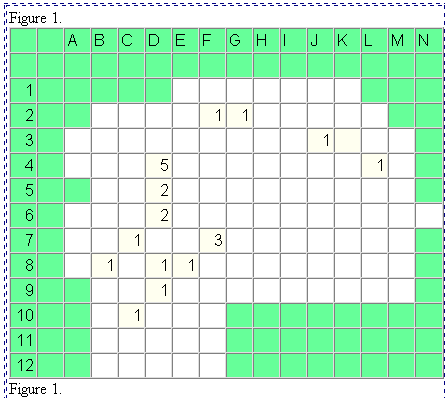
figure on the left shows the spatial distribution of
the number
of individuals accepting a particular innovation after
one year of
observation
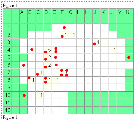
(Hägerstrand, p. 380). The figure on the right
shows a map of
the same region and of the pattern of acceptors after
two years--based
on actual evidence. Notice that the pattern at a later
time shows both
spatial expansion and spatial infill (more
concentrated use and greater
density per unit of land area). These two latter
related concepts are
also enduring
ones and they appear over and over again in spatial
analysis---as well
as in
planning at municipal and other levels.
Might it have been
possible to make an educated guess, from Figure 1
alone, as to how the news of the innovation would
spread? Or might one
develop Figure 2 from the Figure 1 using
some replicable, systematic process?
What are the
intellectual and deep challenges to modelling such
process?
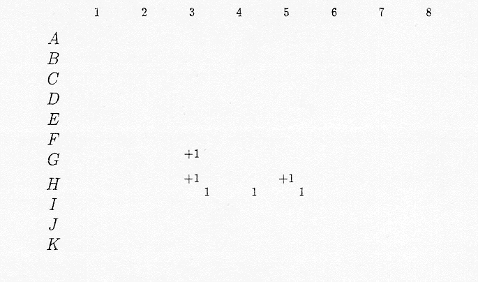
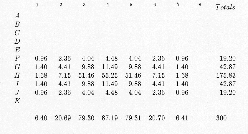
The numbers in the floating grid, used with a set of four digit random numbers, will be used to determine likely location of new adopters. It is shown in enlarged form on the right of Figure 3. Notice that cells close to the center of the grid contain a wider interval of four digit numbers than do those near the edge. Hence, it is more likely that a random number will fall within in an interval near the center than near the edge. This numerical pattern reflects the idea that an individual is more likely to communicate with someone nearby than with someone far away (Tobler's Law); velocity of diffusion is expressed in terms of probability of contact. That is, the assignment of four digit numbers reflects the probability of contact; in this case that assignment is symmetric, but asymmetric assignment might reflect decisions about boundaries and other physical or human features. In Figure 3, there are 22 initial adopters and thus 22 random numbers. Different sets of random numbers produce results that are different from each other in terms of detail of distribution but probably not in terms of general pattern of clustering, infill, and spatial extension. This assumption regarding distance and probability of contact is reflected in the assignment of numerals within the grid--there are the most four digit numbers in the central cell, and the fewest in the corners. The floating grid partitions the set of four digit numbers {0000, 0001, 0002, ..., 9998, 9999} into 25 mutually disjoint subsets. The grid together with the sets of numbers is referred to (by Hägerstrand and others) as the Mean Information Field (MIF).
Figure
4 demonstrates the detail of using the Mean Information
Field to
generate a simulation of the diffusion of an
innovation. Center
the floating grid on F2. The first random number
(from Figure 3)
is 6248 and it lies
in the center square of the MIF. So in the simulation,
the acceptor
in F2 finds another acceptor nearby in F2. Record that
simulated
acceptor
as a red dot. Together with the original adopter, there
are now two
adopters
in this cell. Move the MIF over and center it on
the next cell
with a numeral/adopter (as suggested in the animation in
Figure 3) and
repeat the procedure using the
next random number in the sequence. The animation
of Figure 4
shows the use of the entire set of random numbers in
Figure 3 and the
consequent simulated pattern of new adopters.
Figure 5 shows a
static view and illustrates issues associated with edge
effect problems.
While
the spatial pattern simulated is discrete, it is based
on underlying
continuous mathematics. The construction of the
MIF assumes,
based on empirical evidence, that the frequency of
social contact
(communication, migration) per square kilometer falls
off or decays
with distance. And, this idea is captured
easily with a
distance decay curve, a continuous curve, with units
on the x-axis
expressed in terms of kilometers and on the y-axis in
terms of the
number of migrating households per square
kilometer. More
detailed information on the mechanics of construction
is available at a
variety of locations including at the following linked site. Contemporary Vision Two
toolkits that were not available to Hägerstrand for
his analysis of the
diffusion of an innovation were fractal geometry and
Geographic
Information Systems (GIS) software. We
consider superimposing
these two tools on the classical idea. A
Space-Filling Vision of Diffusion
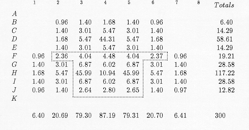
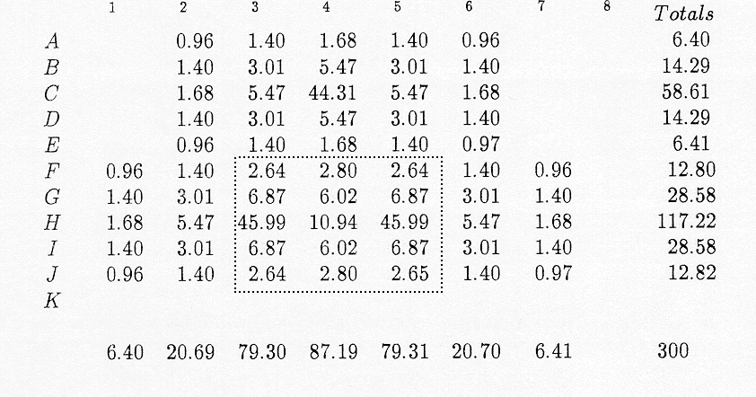
Given a view of a gridded locale in
the style of Hägerstrand (Figure 6), along with an
associated 5-by-5
MIF (Figure 7) with numerical entries expressed
as percentages of
the numbers from Figure 3. Thus, for example,
the central cell
contains 44.31 percent of the four digit numbers and
the likelihood
that an individual in that cell will contact another
within that cell
is 44.31 percent. Probabilities of the
likelihood of contact
simulate the spread of knowledge of the innovation
over time.
Over time, the information will spread, gaps will fill
in and,
eventually, the population will become saturated with
the
information. Figure 6 shows a very simple
pattern of initial
adopters, coded as '1' in three cells: H3, H4,
and H5. The
first generation of adopters adds three more adopters,
one each in
cells H3, G3, and H5, using the first three random
numbers from Figure
3: H3 goes to H3 from 6248; H4 goes to G3 from
0925; and, H5 goes
to H5 from 4997.
Because of the weighting of the assignment of
probabilities, clearly
different initial distributions of adopters will lead
to different
outcomes of specific locations, even though there may
be general
pattern similarities.
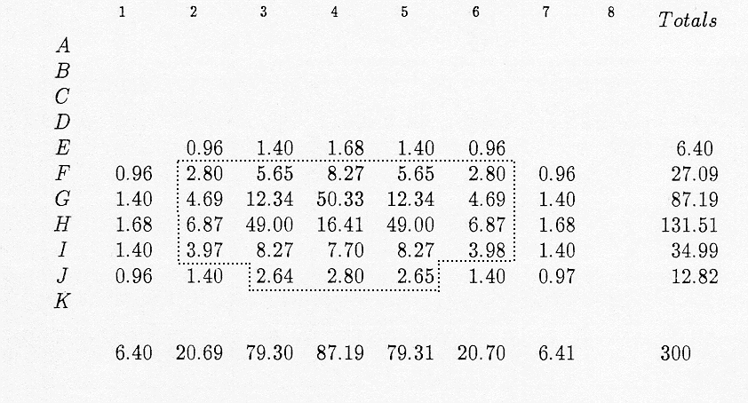
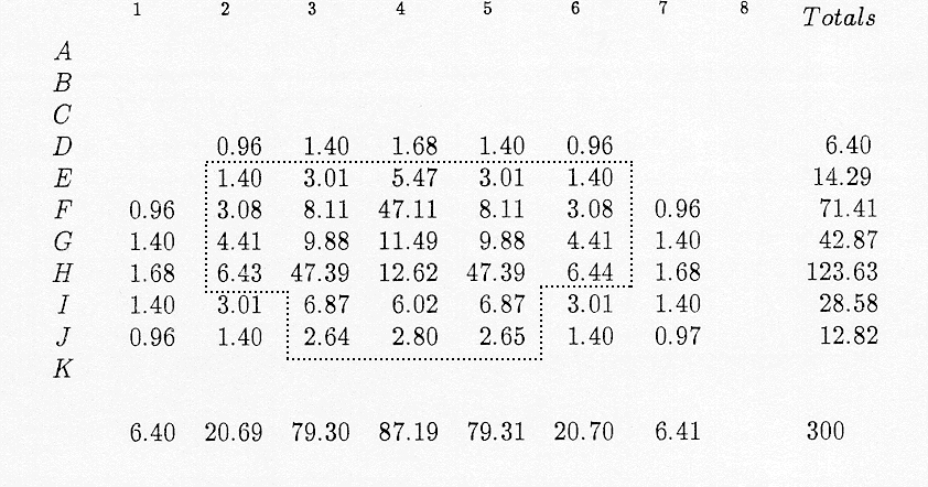
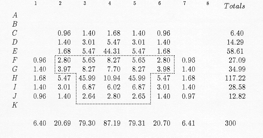
Independent of how many generations are calculated using this procedure, the pattern of "filling in" of new adopters is heavily influenced by the shape of the set of original adopters. Indeed, over time, knowledge of the innovation diffuses slowly initially, picks up in speed of transmission, tapers off, and eventually the population becomes saturated with the knowledge. Typically, this process is characterterized as a continuous phenomenon using a differential equation of inhibited growth that has as an initial supposition that the population may not exceed M, an upper bound, and that P(t), the population P at time t, grows at a rate proportional to the size of itself and proportional to the fraction left to grow (Haggett et al., 1977; Boyce and DiPrima, 1977). An equation such as dP(t) / dt = kP9t)(1-(P(t)/M)) serves as a mathematical model for this sort of growth in which k>0 is a growth constant and the fraction (1-(P(t)/M) acts as a damper on the rate of growth (Boyce and DiPrima, 1977). The graph of the equation is an S-shaped (sigmoid) logistic curve with horizontal asymptote at P(t)=M and inflection point at P(t)=M/2. When dP/dt >0 the population shows growth; when d2P/dt2 > 0 (below P(t) = M/2) the rate of growth is increasing; when d2P/dt2 < 0 (above P(t) = M/2) the rate of growth is decreasing. The differential equation model thus yields information concerning the rate of change of the total population and in the rate of change in growth of the total population. It does not show how to determine M; the choice of M is given a priori. Iteration of the Hägerstrand procedure gives a position for M once the procedure has been run for all the generations desired. For, it is a relatively easy matter to accumulate the distributions of adopters and stack them next to each other, creating an empirical sigmoid logistic curve based on the simulation (Haggett et al., 1977). Finding the position for the asymptote (or for an upper bound close to the asymptotic position) is then straightforward. Neither the Hägerstrand procedure nor the inhibited growth model provides an estimate of saturation level (horizontal asymptote position) (Haggett, et al., 1977) that can be calculated in the measurement of the growth. The fractal approach suggested below offers a means for making such a calculation when self-similar hierarchical data are involved; allometry is a special case of this procedure (Mandelbrot, 1983; Michigan Inter-University Community of Mathematical Geographers). The reasons for wanting to make such a calculation might be to determine where to position adopter 'seeds' in order to produce various levels of innovation saturation. The following example illustrates how a fractal/space filling approach, based on self-similarity, can offer measures, at the outset and based only on the positions of the initial adopters, of eventual saturation. To follow the mechanics of the process, suppose, in Figure 8a, that the grid of Figure 7 is superimposed and centered on the original adopter in cell H3. A probability of 3.01% is assigned to the likelihood for contact from H3 to G4. When the grid is superimposed and cnetered on the original adopter in H4, there is a 5.47% likelihood for contact from H4 to G4. And, when the grid is superimposed and centered on the original adopter in H5, there is once again a 3.01% likelihood for contact from H5 to G4. Therefore, the percentage likelihood of a new first-generation adopter in cell G4, given this initial configuration of adopters, is the sum of the percentages dificed by the number of initial adopters, or 11.49/3. For ease in serting fractions into a grid, only the numerator, 11.49, is shown as the entry (Figure 8a). Then, the procedure is repeated for each cell in configuration. It is only in zones of overlap of the grid, as it moves from one original adopter to the next that the entries in this table will differ from those in the MIF of Figure 7. This zone of overlap, of at least two of the MIF positions, is called the zone of interaction. In Figure 8a, the zone of interaction concides with the blue rectangle represening the MIF centered on the middle adopter. Then, adjust the position of an original adopter. The center adopter, in H4 will be moved, one unit toward the top in each of Figures 8b, 8c, 8d, 8e, and 8f. The resulting configurations, row and column totals (with column totals constant and row total patterns changing), and zones of interaction are shown in the sequence of figures below. In the last figure, the MIF of the center adopter has now moved out of the picture and no longer intersects the other two.
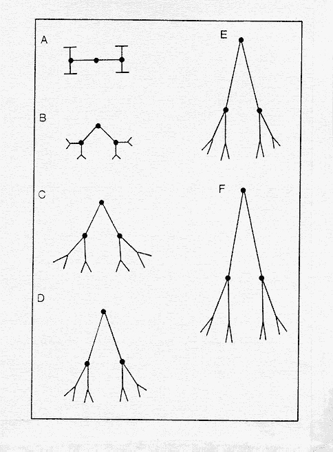
As the central adopter cell moves
toward the top, note that naturally the associated
pattern within the
interaction zone preserves the same bilateral symmetry
(up to
truncation) as the underlying root MIF. Thus,
any configuration
characterizing the pattern in this sequence of figures
should also
exhibit bilateral symmetry. One such form is a
tree. In
fact, if one thinks of each of the three initial
adopter cells as a
point centered in a cell of 1 unit side, then the
three cells in Figure
8a might be represented as a linear pattern, suggested
in Figure 9a,
top. In that image, view the tree on vertices
H3, H4, and H5 as a
generator for a self-similarity sequence (as suggested
by the
arms formed in two successive stages in that
figure). In a
similar manner, other trees are generated for each
movement of the
central original adopter, with Figure 9b derived from
Figure 8b, and so
forth.
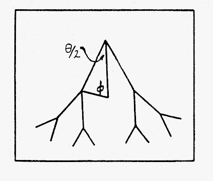
Table 1. Calculation of θ
for each of the distributions of original adopters
in Figure 8.
Table 2. Thus, a measure that reflects the
degree of space-filling, based only on the pattern of
original
adopters, can follow from use of fractal
iteration. It
fulfills the sought purpose of being able to offer a
measure of
eventual saturation, at the outset of a
simulation. It is not
unique and is dependent on generator formulation (as
such things must
be); but it adds and extra dimension to the previous
analysis and it is
possible because advances in technology in the latter
part of the
twentieth century permitted visualization of geometric
form previously
"seen" only through notation. GIS
software
Fractal
geometry offered one great toolkit for visualization and
consequent
solution to new or existing problems; Geographic
Information Systems
software offers yet another. The following
example employs
GIS software (Esri) to integrate the geographic concept
of diffusion
with the business concept of market competition in a
spatial
context. Lists of radio stations were researched,
compiled, and
then mapped in ArcGIS (Figure 11). When suitable
marker symbols were introduced, it became
straightforward to see the
radio catchment areas for the Kansas City Royals
baseball team and for
the St. Louis Cardinals baseball team. Big
businesses wishing to
direct the attention of baseball fans to particular
products, perhaps
with a regional emphasis, need look no further than
toward this sort of
map!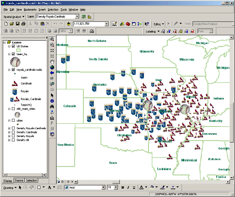 Figure 11. Radio catchment regions of St. Louis Cardinal and Kansas Royal baseball broadcasts. |
|||||||||||||||||||||||||||||||||||||||||||||||||||||||||||||||||||||||||||||||||||||||||||||||||||||||||||||||||||||||||||||||||||||||||||||||||||||||||||||||||||||||||||||||||||||||||||||||||||||||||||||||||||||||||||||||||||||||||||||||||||||||||||||||||||||||||||||||||||||||||||||||||||||||||||||||||||||||||||||||||||||||||||||||||||||||||||||||||||||||||||||||||||||||||||||||||||||||||||||||||||||||||||||||||||||||||||||||||||||||||||||||||||||||||||||||||||||||||||||||||||||||||||||||||||||||||||||||||||||||||||||||||||||||||||||||||||||||||||||||||||||||||||||||||||||||||||||||||||||||||||||||||||||||||||||||||||||||||||||||||||||||||||||||||||||||||||||||||||||||||||||||||||||||||||||||||||||||||||||||||||||||||||||||||||||||||||||||||||||||||||||||||
| These
items illustrate some of our educational and
scholarly
interests
and suggest directions for future work.
Some interactive
examples
are
simple but not necessarily "easy"; indeed,
"simple" is often the
hallmark of elegance that piques
curiosity and stimulates both the motivation
to learn eagerly and
the imagination to pursue new directions.
As
with Faulkner's
'man', fundamental concepts such as diffusion will not
merely
endure, they will prevail: from the
classical to the
contemporary, in
theory and
in practice...all independent of associated toolkit
transformations. |
|||||||||||||||||||||||||||||||||||||||||||||||||||||||||||||||||||||||||||||||||||||||||||||||||||||||||||||||||||||||||||||||||||||||||||||||||||||||||||||||||||||||||||||||||||||||||||||||||||||||||||||||||||||||||||||||||||||||||||||||||||||||||||||||||||||||||||||||||||||||||||||||||||||||||||||||||||||||||||||||||||||||||||||||||||||||||||||||||||||||||||||||||||||||||||||||||||||||||||||||||||||||||||||||||||||||||||||||||||||||||||||||||||||||||||||||||||||||||||||||||||||||||||||||||||||||||||||||||||||||||||||||||||||||||||||||||||||||||||||||||||||||||||||||||||||||||||||||||||||||||||||||||||||||||||||||||||||||||||||||||||||||||||||||||||||||||||||||||||||||||||||||||||||||||||||||||||||||||||||||||||||||||||||||||||||||||||||||||||||||||||||||||
| REFERENCES Arlinghaus, Sandra L. 1990. "Beyond the Fractal." Solstice: An Electronic Journal of Geography and Mathematics. Volume I, No. 1. Ann Arbor: Institute of Mathematical Geography. Volume also reprinted as IMaGe Monograph 13. Both openly available at http://www.imagenet.org/ as well as in Deep Blue, the persistent electronic archive of The University of Michigan. Arlinghaus, Sandra and Kerski, Joseph. 2010. MatheMaPics. Solstice: An Electronic Journal of Geography and Mathematics. Volume XXI, No. 1. Ann Arbor: Institute of Mathematical Geography. Also in Deep Blue, as above. Arlinghaus, Sandra and Kerski, Joseph. 2013. Spatial Mathematics: Theory and Practice through Mapping. Boca Raton: CRC Press, a Division of Taylor and Francis. Blass, A. and Harary, F. Properties of almost all graphs and complexes. Journal of Graph Theory 3 (1979), 225-240. Boyce, W. E. and DiPrima, R. C. 1977. Elementary Differential Equations. New York: Wiley. Guidelines for Geographic Education, Elementary and Secondary Schools. 1984. National Council for Geographic Education and Association of American Geographers. Hägerstrand, Torsten. 1967. Innovation Diffusion as a Spatial Process. Translated by Allan Pred. Chicago: University of Chicago Press. Haggett , P.; Cliff, A. D.; and Frey, A. 1977. Locational Analysis in Human Geography. New York: Wiley. Kerski, Joseph. 2008. "Baseball Radio Station Analysis." http://edcommunity.esri.com/software-and-data/Lessons/B/Baseball_Radio_Station_Analysi Kerski, Joseph. 2009. "Making Your Point with Marker Symbols." http://www.esri.com/news/arcuser/0109/files/marker.pdf Mandelbrot, B. 1983. The Fractal Geometry of Nature. New York: W. H. Freeman. Marble, Duane. Association of American Geographers, April 2013. Geospatial and Geographical analysis. An example for kids Michigan Inter-University Community of Mathematical Geographers, series reprinted available online in Deep Blue, the persistent archive of The University of Michigan. Tobler W., (1970) "A computer movie simulating urban growth in the Detroit region". Economic Geography, 46(2): 234-240. |
|||||||||||||||||||||||||||||||||||||||||||||||||||||||||||||||||||||||||||||||||||||||||||||||||||||||||||||||||||||||||||||||||||||||||||||||||||||||||||||||||||||||||||||||||||||||||||||||||||||||||||||||||||||||||||||||||||||||||||||||||||||||||||||||||||||||||||||||||||||||||||||||||||||||||||||||||||||||||||||||||||||||||||||||||||||||||||||||||||||||||||||||||||||||||||||||||||||||||||||||||||||||||||||||||||||||||||||||||||||||||||||||||||||||||||||||||||||||||||||||||||||||||||||||||||||||||||||||||||||||||||||||||||||||||||||||||||||||||||||||||||||||||||||||||||||||||||||||||||||||||||||||||||||||||||||||||||||||||||||||||||||||||||||||||||||||||||||||||||||||||||||||||||||||||||||||||||||||||||||||||||||||||||||||||||||||||||||||||||||||||||||||||
|
.

Solstice:
An Electronic Journal of Geography and
Mathematics, |
|
Congratulations to all Solstice contributors. |
| Remembering
those who
are gone now but who contributed in various ways to Solstice or
to IMaGe
projects, directly or indirectly, during the first 25
years of IMaGe: Allen K. Philbrick | Donald F. Lach | Frank Harary | H. S. M. Coxeter | Saunders Mac Lane | Chauncy D. Harris | Norton S. Ginsburg | Sylvia L. Thrupp | Arthur L. Loeb | George Kish | |