Making It Clear: The Importance of Transparency
Sandra Lach Arlinghaus
Fractal Earth
Download this associated kml file for the first section.
SECTION 1: SELF-ECLIPSING TILES ON THE GLOBE
| In the chapter on Escher/Barr Earth, it was noted that polygons on the surface experience a "self-eclipsing" effect when they are spun around the globe, as they move from front to back. The extent to which the eclipsing effect occurs appears to depend on where they make the front to back transition. In Figure 1, the Koch Island, a classical fractal curve, is shown at a fairly simple state of fractal iteration. Three copies of that curve are stacked up at 50,000 meters (yellow), 100,000 meters (red), and 150,000 meters (purple). They are stacked on a white base tile that is clamped to the ground on the Google Globe (with the terrain switched off). The figure is animated to show the effect of moving this stacked Koch tile in a due east-west direction. |
 Figure 1. Animation of an East-West tour of a Koch Island tile (low in the fractal iteration sequence). Download the associated kml file and play the EW tour or move the tile around freely to study self-eclipsing effects as the tile moves from front to back of the Google Globe. |
| Figures
2a,
2b, and 2c show Koch Island tours (Koch's Tours?)
along great
circle routes at headings of 45 degrees, 67 degrees,
and 90 degrees
respectively. The interval between successive
screen shots in the
animation is 20 degrees of longitude. The images
in Figure 1 and
Figure 2 all suggest that the self-eclipsing effect is
strong near the
horizon, only. They also suggest that there may be variation, depending on heading, as to when the white base comes into view on the back side. There is a region of "umbra" in which the non-white stack is visible near the edge but none of the white is visible. There is a region of "penumbra" in which only part of the white base is visible. Once the stack is beyond the penumbra on the backside, a sort of Moiré effect from the translucent tile reveals the underlying graticule on which the projection is based. The projection appears to be an orthographic projection: a perspective projection from sphere to plane in which the center of projection is from a point at infinity. The center of the Koch Island tile in initial position, and its antipodal point, form a central axis for these views of the circulating tiles independent of heading. |
 Figure 2a. Animation of an 45 degree heading great circle tour of a Koch Island tile (low iteration). Download the associated kml file and play the 45 degree tour or move the tile around freely to study self-eclipsing effects as the tile moves from front to back of the Google Globe. |
 Figure 2a. Animation of a 67 degree heading great circle tour of a Koch Island tile (low iteration). Download the associated kml file and play the 67 degree tour or move the tile around freely to study self-eclipsing effects as the tile moves from front to back of the Google Globe. |
 Figure 2c. Animation of an 90 degree heading great circle tour of a Koch Island tile (low iteration). Download the associated kml file and play the 90 degree tour or move the tile around freely to study self-eclipsing effects as the tile moves from front to back of the Google Globe. |
| A
simple shot of the Grid, from a polar perspective
(Figure 3) shows
the
characteristic spacing of the orthographic graticule
with great circles
becoming more
closely spaced as one moves away from the center
(which is assumed
along the Earth's polar axis--conversation wtih
Michael Weiss-Malik
at lunch (October 23, 2008) in which he noted that the
Google Earth
singularities are at
the Earth's poles). Thus,
zoom length can be "infinite." The map "looks"
like the
globe. The central-axis property revealed
by the Moiré
effect
on the tiles in
Figures 1 and 2 is clearly the case for all headings,
and not just
those tested, if the underlying
projection is indeed orthograpic. |
 Figure 3. Apparent orthographic graticule serving as the projection base for the Google Globe. |
| When
the vantage point is varied the location of the umbra
and penumbra will
vary. Consider the
images in Figure 4: they show views of the Koch
Island tile all
at 110
degrees East Longitude at varying values of Latitude
(10, 20, 30, 40,
50, 60, 70, 80, 89). The white base of the tile
comes into view
at
variable positions. One might speculate that
perhaps the crossing
of a
singular point is the cause: the software
produces errors when
trying
to enter (110, 90). Or one might be tempted to
think that the
crossing of tiles of the underlying quadtree data
structure alters the
location of the umbra and penumbra. There are
experiments,
suitably
named, also in the kml file for download. Those
reasons, while
perhaps
natural concerns, appear not to have much merit.
|
 Figure 4. Koch Island tiles along the horizon. |
| What
matters is primarily
the position of the observer: much as it does in
a solar or lunar
eclipse. Figure 5a shows the position for
(50,110) from the
animation
above. Figure 5b shows the same tile, in the
same position,
viewed
from the North pole. Because this latter vantage
point is along
the axis
of
the
underlying orthographic projection, there is no
variation, of the sort
in Figure 4, in position of umbra and
penumbra. Use the kml
file to have multiple views and to see this effect
clearly for any
location. |
 Figure 5a. Lateral view of the Koch Island tile located at (50, 110). |
 Figure 5b. Polar view of the Koch Island tile located at (50, 110). |
Questions
for
further thought:
|
SECTION 2: SELF-SIMILAR TILES ON THE GLOBE-- A HEXTREE BASIS?
| Apparently,
the
quadtree (or perhaps octree?) is the basis for the
data structure
underlying Google Earth (Mano Marks, workshop
communication, October
23, 2008). A visual representation of these
structures
has a fractal-like form in which the same pattern is
applied to
partition data at successively more local
scales. Broadly viewed, one might then wonder if some sort of geometry configuration, based on close-packings, might be an interesting way to split up tiles on the surface of the sphere. Hexagons form the tightest close-packing. A number of years ago, Azriel Rosenfeld noted, at an American Mathematical Society meeting, that hexagonal pixels would make sense if one were trying to optimize spatial content on a computer screen. He noted, however, that printer technology was based on a rectilinear grid and so the requirements for a skewed-looking printer were not appealing to printer manufacturers. Later essays (see references) note various uses and theoretical findings involving hexagonal packings. Figures 6a, 6b, and 6c, show three different close packings with layers of successively smaller polygon nets oriented in a variety of patterns--they determine, in a general sense, all others. Each may be fractally generated and each is listed with its fractal dimension (space-filling capability). |
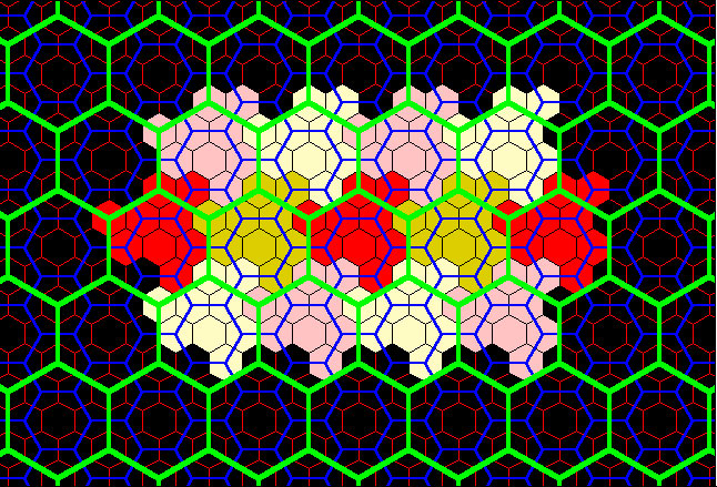 Figure 6a. Principle of 3. Fractal generation procedure suggested by tiling pattern. Fractal dimension when iteration is carried out infinitley is: 1.2618595 |
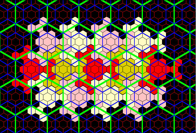 Figure 6b. Principle of 4. Fractal generation procedure suggested by tiling pattern. Fractal dimension when iteration is carried out infinitley is: 1.5849625 |
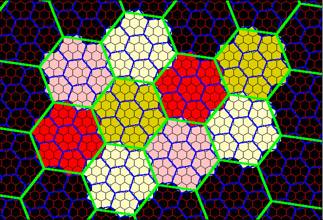 Figure 6c. Principle of 7. Fractal generation procedure suggested by tiling pattern. Fractal dimension when iteration is carried out infinitley is: 1.1291501 |
| One might imagine each of these as a "hextree" on which to hang spatial information in association with the material about the Earth already present in Google Earth. Figure 7a shows the pattern of Figure 6a applied to the Google Globe. Figure 7b shows that pattern in association with the underlying terrain. If the tiles could be made to all be the same size, and not scaled to the lat/long graticule, then distant tiles brought into focus would enlarge--that feature is often a desirable factor when thinking of navigating in real Earth based space. What looks small on the horizon becomes larger as it is approached! |
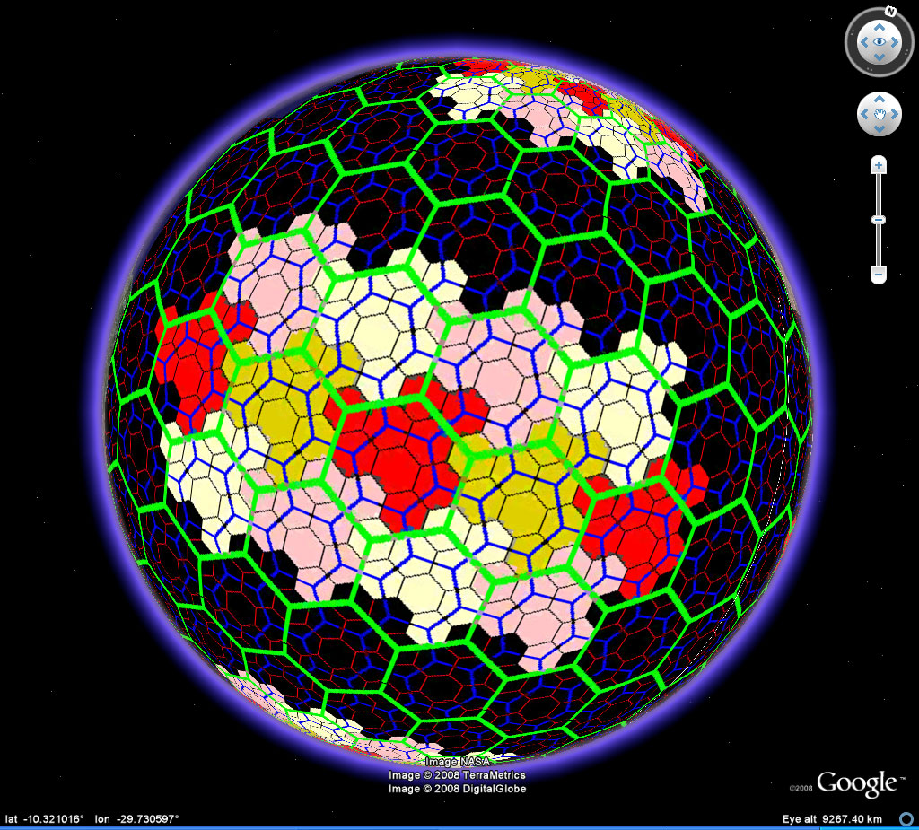 Figure 7a. One scheme for creating close-packed regions. Fractal dimension: 1.2618595 |
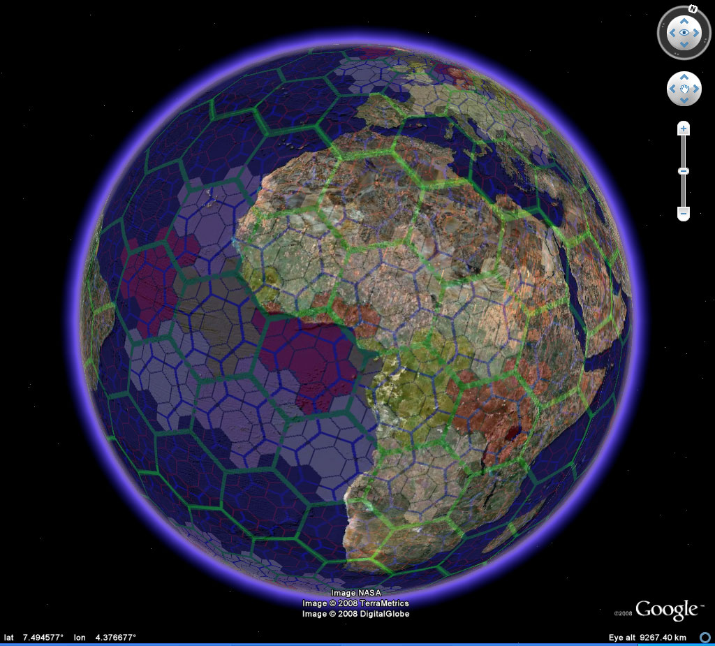 Figure 7b. Regions in association with topography and other terrestrial and oceanic information. Transparency can be important in turning theory into practice. |
Questions
for
further thought:
|
REFERENCES:
Arlinghaus, Sandra L. "Fractals take a central place," Geografiska Annaler, 67B, (1985), pp. 83-88. Journal of the Stockholm School of Economics. 1985.
Arlinghaus, Sandra L. "Micro-cell Hex-nets" Solstice: An Electronic Journal of Geography and Mathematics, Institute of Mathematical Geography Previous link is to original TeX code sent around via e-mail; click on the next link to see scanned images of typeset printout made from the TeX file: Micro-cell Hex-nets 1993.
Arlinghaus, Sandra L. and Arlinghaus, William C. "The fractal theory of central place hierarchies: a Diophantine analysis of fractal generators for arbitrary Löschian numbers," Geographical Analysis: an International Journal of Theoretical Geography. Ohio State University Press. Vol. 21, No. 2; pp. 103-121. 1989.
Arlinghaus, Sandra L. and Arlinghaus, William C. "Spatial Synthesis Sampler. Geometric Visualization of Hexagonal Hierarchies: Animation and Virtual Reality." Solstice: An Electronic Journal of Geography and Mathematics, Institute of Mathematical Geography, Ann Arbor, MI. Semi-finalist, Pirelli INTERNETional Award Competition. 2004.
Christaller, Walter. Die zentralen Orte in Süddeutschland: Eine ökonomisch-geographische Untersuchung über die Gesetzmässigkeit der Verbreitung und Entwicklung der Siedlungen mit städischen Funktionen. Jena: Gustav Fischer Verlag. Doktor-Dissertation. 1933.
Dacey, Michael F. The geometry of central place theory. Geografiska Annaler, B, 47, 111-124. 1965.
Lösch, August. The Economics of Location. Yale University Press, 1954.
Marks, Mano (Google), October 23, 2008: Quadtree reference from "advanced" workshop.
Marshall, John U. The Löschian Numbers as a Problem in Number Theory. Geographical Analysis 7, 421-426. 1975.
Nystuen, John D. Personal communication, the importance of tiles on the horizon coming into view to show more. 2008 and earlier.
Weiss-Malik, Michael (Google), October 23, 2008: stated that the underlying projection has singularities at the poles.
Dr. Arlinghaus is Adjunct Professor at The University of Michigan, Director of IMaGe, and Executive Member, Community Systems Foundation.
Solstice: An Electronic
Journal
of Geography and
Mathematics,
Institute of Mathematical Geography, Ann Arbor, Michigan.
Volume XIX, Number 2.
http://www.InstituteOfMathematicalGeography.org/
Persistent URL: http://deepblue.lib.umich.edu/handle/2027.42/58219
Volume XIX, Number 2.
http://www.InstituteOfMathematicalGeography.org/
Persistent URL: http://deepblue.lib.umich.edu/handle/2027.42/58219